Exact2Pass

Last Update 1 day ago Total Questions : 26
The Excel 2016 Expert: Interpreting Data for Insights content is now fully updated, with all current exam questions added 1 day ago. Deciding to include 77-728 practice exam questions in your study plan goes far beyond basic test preparation.
You'll find that our 77-728 exam questions frequently feature detailed scenarios and practical problem-solving exercises that directly mirror industry challenges. Engaging with these 77-728 sample sets allows you to effectively manage your time and pace yourself, giving you the ability to finish any Excel 2016 Expert: Interpreting Data for Insights practice test comfortably within the allotted time.
You have been a manager of a band for the past year. You are reviewing the data you have about the merchandise that was sold at all of the concerts.
Task 4:
Exhibit:
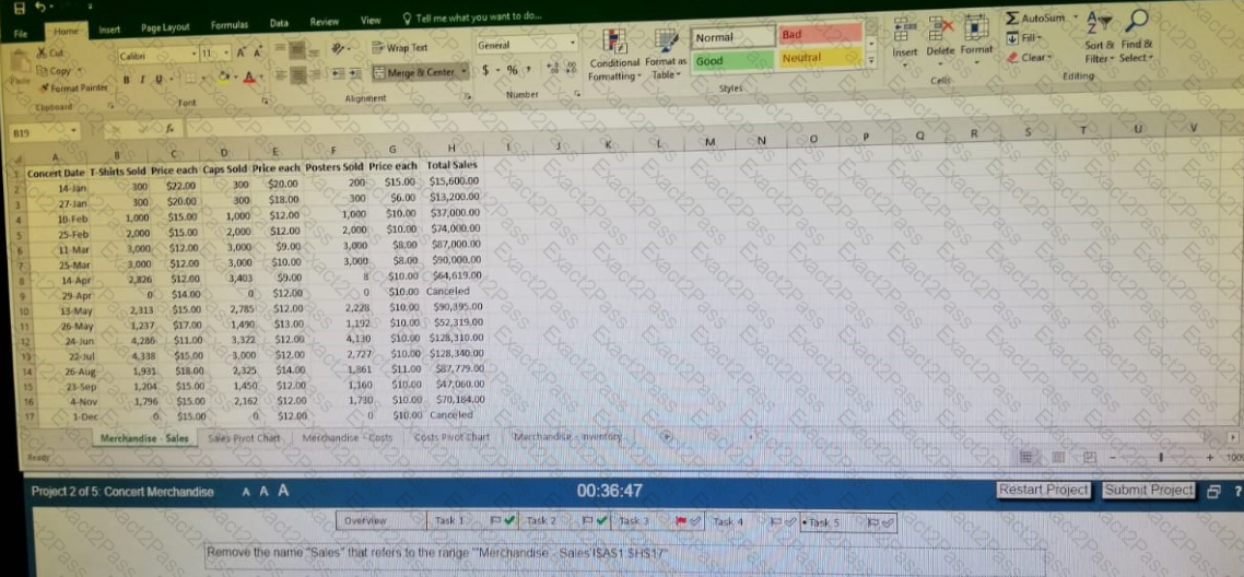
Remove the name “Sales” that refers to the range “Merchandise-Sales’ISAS1 SHS17”
Exhibit:
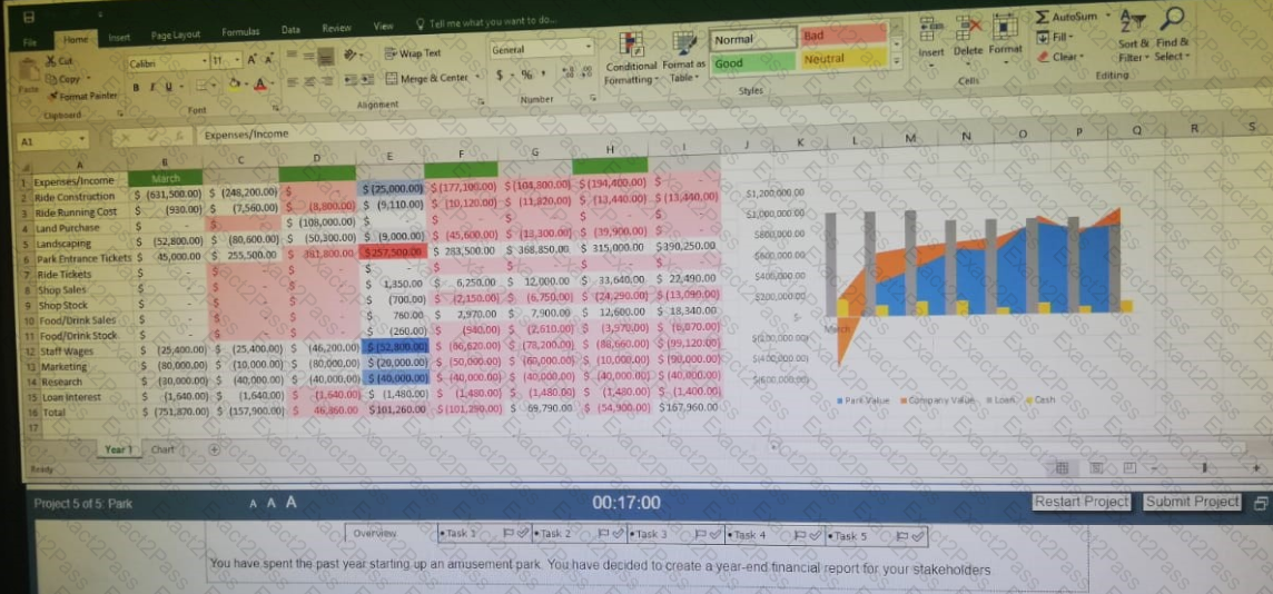
You have spent the past year starting up an amusement park. You have decided to create a year end financial report for your stakeholders.
Task 3:
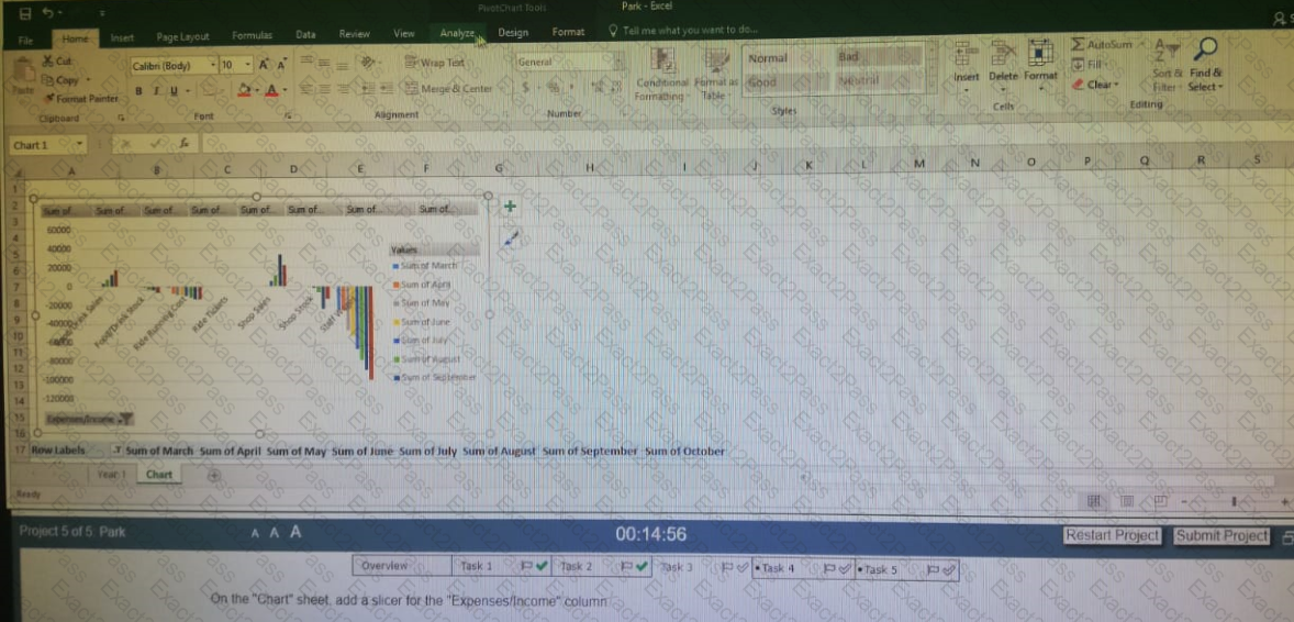
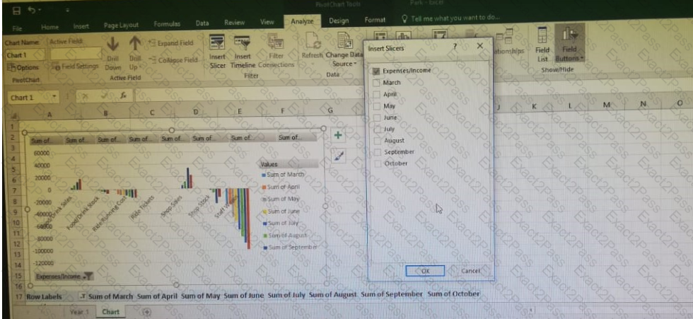
On the “Chart” sheet add a slicer for the “Expense/Income” Column
Exhibit:
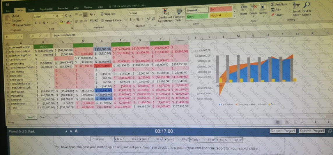
You have spent the past year starting up an amusement park. You have decided to create a year end financial report for your stakeholders.
Task 5:
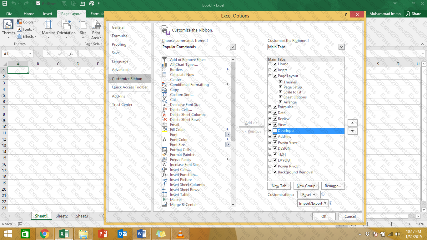
Show the Developer tab on the ribbon.
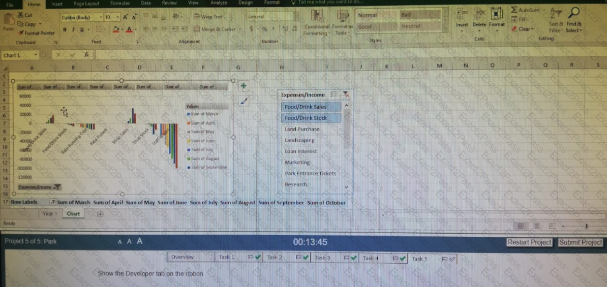
Exhibit:
Task 5:
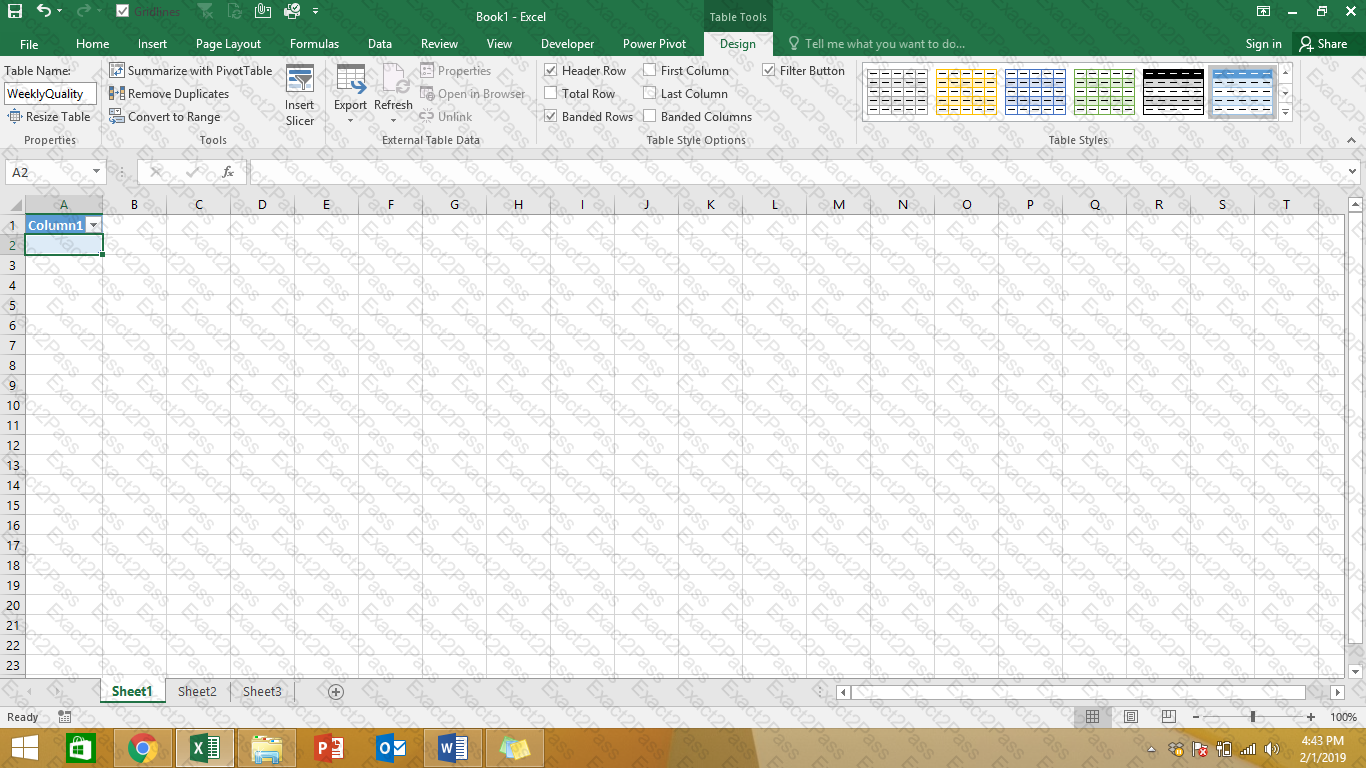
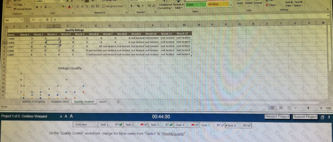
On the “Quality Control” worksheet change the table name from “Table3” to WeeklyQuality”.
Exhibit:
Task 1:
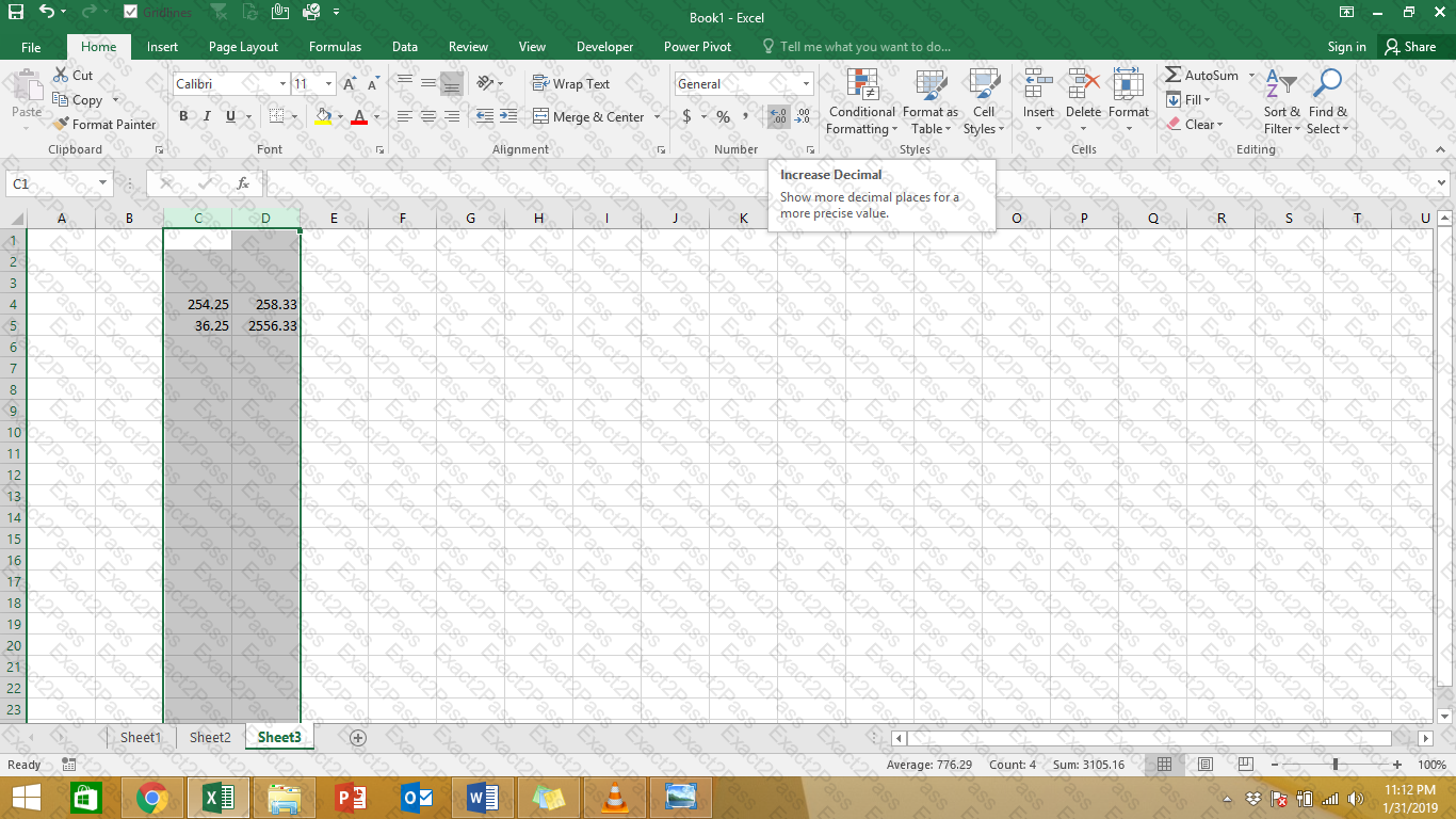
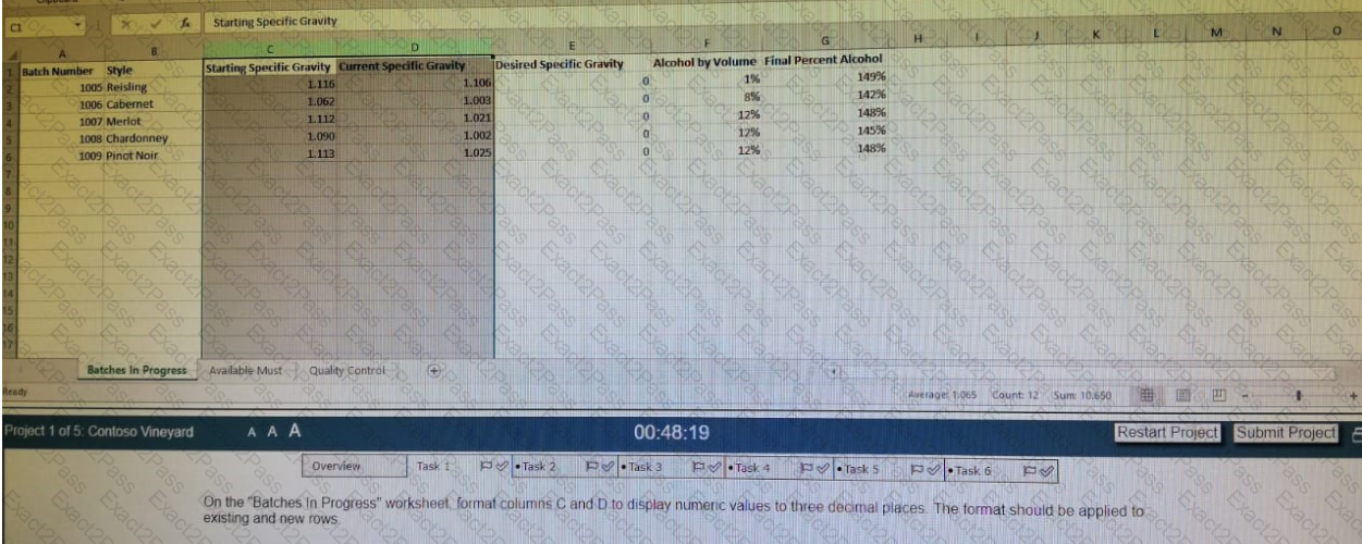
On the “Batches in progress” worksheet format columns C and D to display numeric values to three decimal places. The format should be applied to existing and new row
Exhibit:
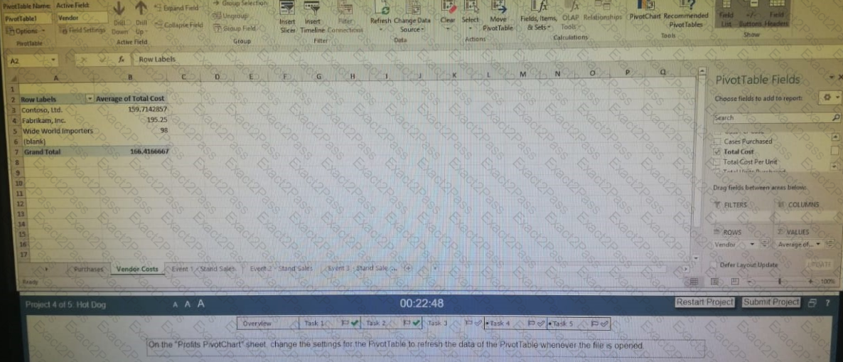
You are an accountant for an event stadium. You have created a workbook to keep track of the four vendors that are available at the stadium.
Task 4:
Exhibit:
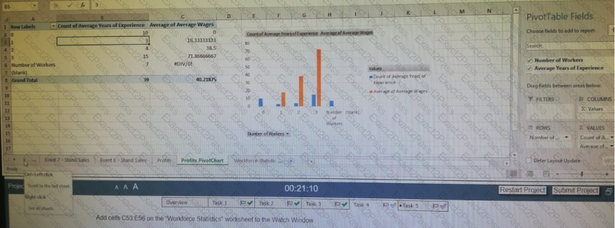
Add cells C53 E56 on the “Workforce Statistics” worksheet to the Watch Window.
You are an accountant for an event stadium. You have created a workbook to keep track of the four vendors that are available at the stadium.
Task 2:
Create a PivotTable in Cell A2 of the “Vendor Costs” worksheet based on cells C3 K19 on the “Purchases” worksheet to show the average of the total cost for each vendor. Display each vendor on a row.